Understanding Memory
Last updated on 2025-01-30 | Edit this page
Estimated time: 30 minutes
Overview
Questions
- How does a CPU look for a variable it requires?
- What impact do cache lines have on memory accesses?
- Why is it faster to read/write a single 100mb file, than 100 1mb files?
Objectives
- Able to explain, at a high-level, how memory accesses occur during computation and how this impacts optimisation considerations.
- Able to identify the relationship between different latencies relevant to software.
Accessing Variables
The storage and movement of data plays a large role in the performance of executing software.
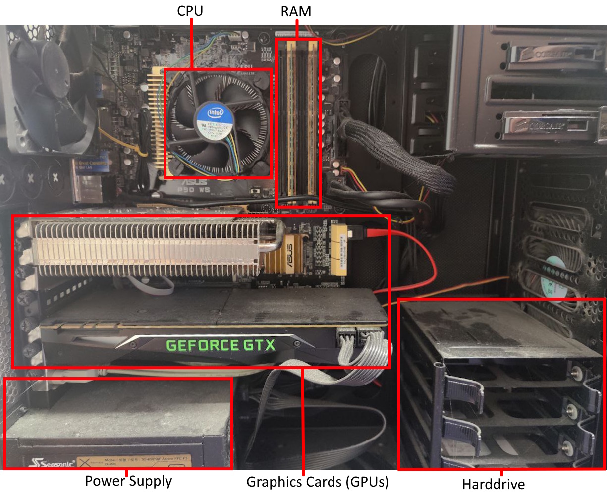
Modern computers have a single CPU with multiple cores, each capable of working on tasks at the same time. Data used by programs is stored in RAM, which is faster than hard drives or solid-state drives. However, the CPU has even faster memory called caches to access frequently used data quickly.
How the CPU Accesses Data? When the CPU needs to use a variable, it follows these steps:
- Registers: First, the CPU checks its own small, super-fast storage (registers). But it only has room for about 32 variables, so it usually doesn’t find the data here.
- L1 Cache: Next, the CPU looks in the L1 cache. It’s small (64 KB per core) and fast, but it only stores data for a single core.
- L2 Cache: If the variable isn’t in L1, it checks the larger L2 cache, which is shared by several cores. It’s slower than L1 but still faster than RAM.
- L3 Cache: If the variable isn’t in L2, the CPU checks the L3 cache, which is shared by all cores. It’s slower than L2 but bigger.
- RAM: If the variable is still not found, the CPU fetches it from the much slower RAM. The faster the CPU finds the data in the cache, the quicker it can do the job. This is why understanding how the cache works can help make things run faster.
Cache Details: When the CPU pulls data from RAM, it loads not just the variable, but also a full 64-byte chunk of memory called a “cache line.” This chunk often contains nearby variables that might be needed soon. When new data is added to the cache, old data is pushed out.
Because of this, reading a list of data that’s next to each other in memory (like 16 numbers in a row) is much faster than reading scattered data, since the CPU can keep more of it in the cache. To make programs run faster, related data should be stored next to each other in memory. By working with this data while it’s still in the cache, the CPU doesn’t have to go all the way to RAM, which is much slower.
While you don’t need to know all the details of how memory works,
it’s helpful to know that memory locality—keeping related data together
and accessing it in chunks—is key to making programs run faster. 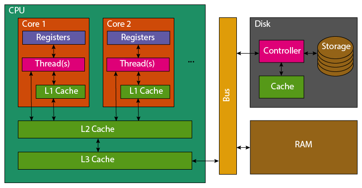
Python as a programming language, does not give you enough control to carefully pack your variables in this manner (every variable is an object, so it’s stored as a pointer that redirects to the actual data stored elsewhere).
However all is not lost, packages such as numpy and
pandas implemented in C/C++ enable Python users to take
advantage of efficient memory accesses (when they are used
correctly).
Accessing Disk
When accessing data on disk (or network), a very similar process is performed to that between CPU and RAM when accessing variables.
When reading data from a file, it transferred from the disk, to the disk cache, to the RAM. The latency to access files on disk is another order of magnitude higher than accessing RAM.
As such, disk accesses similarly benefit from sequential accesses and
reading larger blocks together rather than single variables. Python’s
io package is already buffered, so automatically handles
this for you in the background.
However before a file can be read, the file system on the disk must be polled to transform the file path to it’s address on disk to initiate the transfer (or throw an exception).
Following the common theme of this episode, the cost of accessing randomly scattered files can be significantly slower than accessing a single larger file of the same size. This is because for each file accessed, the file system must be polled to transform the file path to an address on disk. Traditional hard disk drives particularly suffer, as the read head must physically move to locate data.
Hence, it can be wise to avoid storing outputs in many individual files and to instead create a larger output file.
This is even visible outside of your own code. If you try to upload/download 1 GB to HPC. The transfer will be significantly faster, assuming good internet bandwidth, if that’s a single file rather than thousands.
The below example code runs a small benchmark, whereby 10MB is written to disk and read back whilst being timed. In one case this is as a single file, and the other, 1000 file segments.
PYTHON
import os, time

# Generate 10MB
data_len = 10000000
data = os.urandom(data_len)
file_ct = 1000
file_len = int(data_len/file_ct)
# Write one large file
start = time.perf_counter()
large_file = open("large.bin", "wb")
large_file.write(data)
large_file.close ()
large_write_s = time.perf_counter() - start
# Write multiple small files
start = time.perf_counter()
for i in range(file_ct):
    small_file = open(f"small_{i}.bin", "wb")
    small_file.write(data[file_len*i:file_len*(i+1)])
    small_file.close()
small_write_s = time.perf_counter() - start
# Read back the large file
start = time.perf_counter()
large_file = open("large.bin", "rb")
t = large_file.read(data_len)
large_file.close ()
large_read_s = time.perf_counter() - start
# Read back the small files
start = time.perf_counter()
for i in range(file_ct):
    small_file = open(f"small_{i}.bin", "rb")
    t = small_file.read(file_len)
    small_file.close()
small_read_s = time.perf_counter() - start
# Print Summary
print(f"{1:5d}x{data_len/1000000}MB Write: {large_write_s:.5f} seconds")
print(f"{file_ct:5d}x{file_len/1000}KB Write: {small_write_s:.5f} seconds")
print(f"{1:5d}x{data_len/1000000}MB Read: {large_read_s:.5f} seconds")
print(f"{file_ct:5d}x{file_len/1000}KB Read: {small_read_s:.5f} seconds")
print(f"{file_ct:5d}x{file_len/1000}KB Write was {small_write_s/large_write_s:.1f} slower than 1x{data_len/1000000}MB Write")
print(f"{file_ct:5d}x{file_len/1000}KB Read was {small_read_s/large_read_s:.1f} slower than 1x{data_len/1000000}MB Read")
# Cleanup
os.remove("large.bin")
for i in range(file_ct):
    os.remove(f"small_{i}.bin")
Running this locally, with an SSD I received the following timings.
SH
    1x10.0MB Write: 0.00198 seconds
 1000x10.0KB Write: 0.14886 seconds
    1x10.0MB Read: 0.00478 seconds
 1000x10.0KB Read: 2.50339 seconds
 1000x10.0KB Write was 75.1 slower than 1x10.0MB Write
 1000x10.0KB Read was 523.9 slower than 1x10.0MB Read
Repeated runs show some noise to the timing, however the slowdown is consistently the same order of magnitude slower when split across multiple files.
You might not even be reading 1000 different files. You could be reading the same file multiple times, rather than reading it once and retaining it in memory during execution. An even greater overhead would apply.
Latency Overview
Latency can have a big impact on the speed that a program executes, the below graph demonstrates this. Note the log scale!
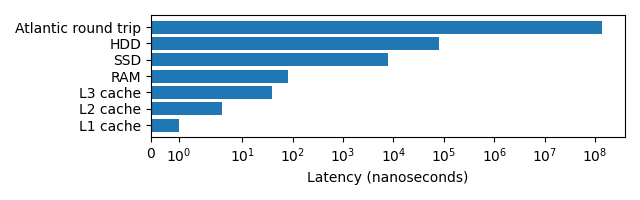
The lower the latency typically the higher the effective bandwidth. L1 and L2 cache have 1TB/s, RAM 100GB/s, SSDs upto 32 GB/s, HDDs upto 150MB/s. Making large memory transactions even slower.
Memory Allocation is not Free
When a variable is created, memory must be located for it, potentially requested from the operating system. This gives it an overhead versus reusing existing allocations, or avoiding redundant temporary allocations entirely.
Within Python memory is not explicitly allocated and deallocated, instead it is automatically allocated and later “garbage collected”. The costs are still there, this just means that Python programmers have less control over where they occur.
The below implementation of the heat-equation,
reallocates out_grid, a large 2 dimensional (500x500) list
each time update() is called which progresses the
model.
PYTHON
grid_shape = (512, 512)

def update(grid, a_dt):
    x_max, y_max = grid_shape
    out_grid = [[0.0 for x in range(y_max)] * y_max for x in range(x_max)]
    for i in range(x_max):
        for j in range(y_max):
            out_xx = grid[(i-1)%x_max][j] - 2 * grid[i][j] + grid[(i+1)%x_max][j]
            out_yy = grid[i][(j-1)%y_max] - 2 * grid[i][j] + grid[i][(j+1)%y_max]
            out_grid[i][j] = grid[i][j] + (out_xx + out_yy) * a_dt
    return out_grid

def heat_equation(steps):
    x_max, y_max = grid_shape
    grid = [[0.0] * y_max for x in range(x_max)]
    # Init central point to diffuse
    grid[int(x_max/2)][int(y_max/2)] = 1.0
    # Run steps
    for i in range(steps):
        grid = update(grid, 0.1)

heat_equation(100)
Line profiling demonstrates that function takes up over 55 seconds of
the total runtime, with the cost of allocating the temporary
out_grid list to be 39.3% of the total runtime of that
function!
OUTPUT
Total time: 55.4675 s
File: heat_equation.py
Function: update at line 4

Line #      Hits         Time  Per Hit   % Time  Line Contents
==============================================================
     3                                           @profile
     4                                           def update(grid, a_dt):
     5       100        127.7      1.3      0.0      x_max, y_max = grid_shape
     6       100   21822304.9 218223.0     39.3      out_grid = [[0.0 for x in range(y_max)] * y_max for x in range(x_m…
     7     51300       7741.9      0.2      0.0      for i in range(x_max):
     8  26265600    3632718.1      0.1      6.5          for j in range(y_max):
     9  26214400   11207717.9      0.4     20.2              out_xx = grid[(i-1)%x_max][j] - 2 * grid[i][j] + grid[(i+1…
    10  26214400   11163116.5      0.4     20.1              out_yy = grid[i][(j-1)%y_max] - 2 * grid[i][j] + grid[i][(…
    11  26214400    7633720.1      0.3     13.8              out_grid[i][j] = grid[i][j] + (out_xx + out_yy) * a_dt
    12       100         27.8      0.3      0.0      return out_grid
If instead out_grid is double buffered, such that two
buffers are allocated outside the function, which are swapped after each
call to update().
PYTHON
grid_shape = (512, 512)

def update(grid, a_dt, out_grid):
    x_max, y_max = grid_shape
    for i in range(x_max):
        for j in range(y_max):
            out_xx = grid[(i-1)%x_max][j] - 2 * grid[i][j] + grid[(i+1)%x_max][j]
            out_yy = grid[i][(j-1)%y_max] - 2 * grid[i][j] + grid[i][(j+1)%y_max]
            out_grid[i][j] = grid[i][j] + (out_xx + out_yy) * a_dt

def heat_equation(steps):
    x_max, y_max = grid_shape
    grid = [[0.0 for x in range(y_max)] for x in range(x_max)]
    out_grid = [[0.0 for x in range(y_max)] for x in range(x_max)]  # Allocate a second buffer once
    # Init central point to diffuse
    grid[int(x_max/2)][int(y_max/2)] = 1.0
    # Run steps
    for i in range(steps):
        update(grid, 0.1, out_grid)  # Pass the output buffer
        grid, out_grid = out_grid, grid  # Swap buffers

heat_equation(100)
The total time reduces to 34 seconds, reducing the runtime by 39% inline with the removed allocation.
OUTPUT
Total time: 34.0597 s
File: heat_equation.py
Function: update at line 3

Line #      Hits         Time  Per Hit   % Time  Line Contents
==============================================================
     3                                           @profile
     4                                           def update(grid, a_dt, out_grid):
     5       100         43.5      0.4      0.0      x_max, y_max = grid_shape
     6     51300       7965.8      0.2      0.0      for i in range(x_max):
     7  26265600    3569519.4      0.1     10.5          for j in range(y_max):
     8  26214400   11291491.6      0.4     33.2              out_xx = grid[(i-1)%x_max][j] - 2 * grid[i][j] + grid[(i+1…
     9  26214400   11409533.7      0.4     33.5              out_yy = grid[i][(j-1)%y_max] - 2 * grid[i][j] + grid[i][(…
10 26214400 7781156.4 0.3 22.8 out_grid[i][j] = grid[i][j] + (out_xx + out_yy) * a_dt- Sequential accesses to memory (RAM or disk) will be faster than
random or scattered accesses.
- This is not always natively possible in Python without the use of packages such as NumPy and Pandas
- One large file is preferable to many small files.
- Memory allocation is not free, avoiding destroying and recreating objects can improve performance.